Photo by Ian Taylor on UnsplashThis tutorial guides you through an analytics use case, analyzing semi-structured data with Spark SQL. We’ll start with the data engineering process, pulling data from an API and finally loading the transformed data into a...

Photo by Ian Taylor on Unsplash

This tutorial guides you through an analytics use case, analyzing semi-structured data with Spark SQL. We’ll start with the data engineering process, pulling data from an API and finally loading the transformed data into a data lake (represented by MinIO). Plus, we'll utilise Docker to introduce a best practice for setting up the environment. So, let’s dive in and see how it’s all done!

Table of contents

Understanding the building blocksSetting up Docker DesktopConfiguring MinIOGetting started with JupyterLabData pipeline: The ETL processAnalysing semi-structured dataCleanup of resources

Understanding the building blocks

This tutorial involves a range of technologies. Before diving into the practical part, let’s grasp each one. We’ll use analogies to make understanding each component easier.

GitHub - sarthak-sarbahi/data-analytics-minio-spark

Imagine you’re a captain setting sail across a vast ocean. In the world of data, this ocean is the endless stream of information flowing from various sources. Our ship? It’s the suite of tools and technologies we use to navigate these waters.

JupyterLab and MinIO with Docker Compose: Just as a ship needs the right parts to set sail, our data journey begins with assembling our tools. Think of Docker Compose as our toolbox, letting us efficiently put together JupyterLab (our navigation chart) and MinIO (our storage deck). It’s like building a custom vessel that’s perfectly suited for the voyage ahead.Fetching data with Python: Now, it’s time to chart our course. Using Python is like casting a wide net into the sea to gather fish (our data). We carefully select our catch, pulling data through the API and storing it in JSON format?—?a way of organizing our fish so that it’s easy to access and use later.Reading and transforming data with PySpark: With our catch on board, we use PySpark, our compass, to navigate through this sea of data. PySpark helps us clean, organize, and make sense of our catch, transforming raw data into valuable insights, much like how a skilled chef would prepare a variety of dishes from the day’s catch.Analytics with Spark SQL: Finally, we dive deeper, exploring the depths of the ocean with Spark SQL. It’s like using a sophisticated sonar to find hidden treasures beneath the waves. We perform analytics to uncover insights and answers to questions, revealing the valuable pearls hidden within our sea of data.

Now that we know what lies ahead in our journey, let’s begin setting things up.

Setting up Docker Desktop

Docker is a tool that makes it easier to create, deploy, and run applications. Docker containers bundle up an application with everything it needs (like libraries and other dependencies) and ship it as one package. This means that the application will run the same way, no matter where the Docker container is deployed?—?whether it’s on your laptop, a colleague’s machine, or a cloud server. This solves a big problem: the issue of software running differently on different machines due to varying configurations.

In this guide, we’re going to work with several Docker containers simultaneously. It’s a typical scenario in real-world applications, like a web app communicating with a database. Docker Compose facilitates this. It allows us to start multiple containers, with each container handling a part of the application. Docker Compose ensures these components can interact with each other, enabling the application to function as an integrated unit.

To set up Docker, we use the Docker Desktop application. Docker Desktop is free for personal and educational use. You can download it from here.

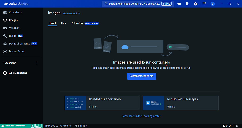Docker Desktop Application (Image by author)

After installing Docker Desktop, we’ll begin with the tutorial. We’ll start a new project in an Integrated Development Environment (IDE). You can choose any IDE you prefer. I’m using Visual Studio Code.

For this guide, I’m using a Windows machine with WSL 2 (Windows Subsystem for Linux) installed. This setup lets me run a Linux environment, specifically Ubuntu, on my Windows PC. If you’re using Windows too and want to enable Docker Desktop for WSL 2, there’s a helpful video you can watch.

Next, we’ll create a docker-compose.yml file in the root directory of our project.

https://medium.com/media/9dcd6a433707451691b11113d15b186f/href

If this is your first time encountering a file like this, don’t fret. I’ll go into more detail about it in the following sections. For now, just run the command docker-compose up -d in the directory where this file is located. This command will initially fetch the Docker images for JupyterLab and MinIO from the Docker Hub.

Results of running the command (Image by author)

A Docker image is like a blueprint or a recipe for creating a Docker container. Think of it as a pre-packaged box that contains everything you need to run a specific software or application. This box (or image) includes the code, runtime, system tools, libraries, and settings?—?basically all the necessary parts that are required to run the application.

Containers are simply running instances of Docker images.

Docker Hub is like an online library or store where people can find and share Docker images.

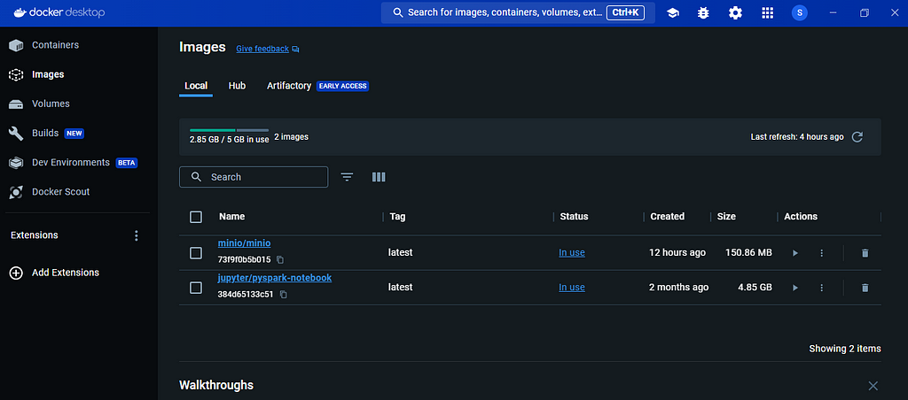Required images have been downloaded (Image by author)

After the images are downloaded, it will launch a container for each image. This process will initiate two containers?—?one for JupyterLab and another for MinIO.

Two containers are running (Image by author)

With the required processes now operational, let’s dive deeper into MinIO and how it’s configured.

Configuring MinIO

MinIO is an open-source object storage solution, specifically designed to handle large volumes and varieties of data. It’s highly compatible with Amazon S3 APIs, which makes it a versatile choice for cloud-native applications.

MinIO is much like using a ‘free’ version of Amazon S3 on your PC.

We’ll utilize MinIO for storing both raw and processed data, mimicking a real-world scenario. Thanks to Docker, we already have MinIO up and running. Next, we need to learn how to use it. But first, let’s revisit the docker-compose.yml file.

The services section in the file outlines the containers we’ll run and the software instances they will initiate. Our focus here is on the MinIO service.

MinIO service in docker-compose.yml file (Image by author)

Let’s break this down.

image: minio/minio tells Docker to use the MinIO image from Docker Hub (the online library of Docker images).container_name: minio1 gives a name to this container, in this case, minio1.ports: - "9000:9000" - "9001:9001" maps the ports from the container to your host machine. This allows you to access the MinIO service using these ports on your local machine.volumes: - /mnt/data:/data sets up a volume, which is like a storage space, mapping a directory on your host machine (/mnt/data) to a directory in the container (/data). This means MinIO will use the /mnt/data directory on your machine to store the data.environment: section sets environment variables inside the container. Here, it's setting the MinIO root user's username and password.command: server /data --console-address ":9001" is the command that will be run inside the MinIO container. It starts the MinIO server and tells it to use the /data directory.

With MinIO’s setup clear, let’s begin using it. You can access the MinIO web interface at http://localhost:9001. On your initial visit, you’ll need to log in with the username (minio)and password (minio123) specified in the docker-compose file.

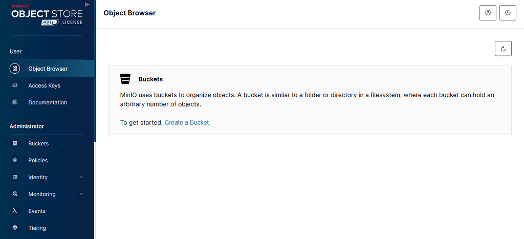MinIO portal (Image by author)

Once logged in, go ahead and create a bucket. Click on ‘Create a Bucket’ and name it mybucket. After naming it, click on ‘Create Bucket.’ The default settings are fine for now, but feel free to read about them on the page’s right side.

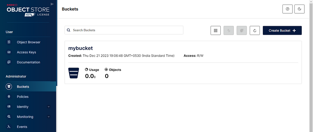Bucket created in MinIO (Image by author)

Well done! We’re now ready to use MinIO. Let’s move on to exploring how we can use JupyterLab.

Getting started with JupyterLab

JupyterLab is an interactive web-based interface that helps us write code, perform analysis on notebooks and work with data. In fact, the JupyterLab image already includes Python and PySpark, so there’s no hassle in setting them up.

JupyterLab service in docker-compose.yml file (Image by author)

First, let’s revisit the docker-compose.yml file to understand the jupyter service.

image: jupyter/pyspark-notebook specifies to use the JupyterLab image that comes with PySpark pre-installed.ports: - "8888:8888" maps the JupyterLab port to the same port on your host machine, allowing you to access it through your browser.

To access its web interface, navigate to the ‘Containers’ tab in the Docker Desktop application. Find and click on the JupyterLab container, labeled jupyter-1. This action will display the container logs.

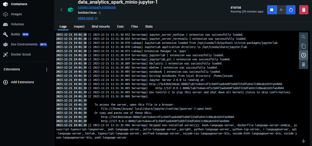JupyterLab container logs (Image by author)

Within these logs, you’ll find a URL resembling this: http://127.0.0.1:8888/lab?token=4f1c9d4f1aeb460f1ebbf224dfa9417c88eab1691fa64b04. Clicking on this URL launches the web interface.

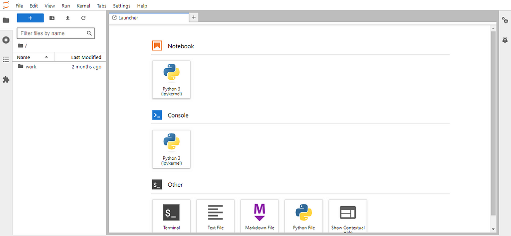JupyterLab web interface (Image by author)

Once there, select the ‘Python 3 (ipykernel)’ icon under the ‘Notebook’ section. This action opens a new notebook, where we’ll write code for data retrieval, transformation, and analysis. Before diving into coding, remember to save and name your notebook appropriately. And there you have it, we’re ready to start working with the data.

Data pipeline: The ETL process

Before diving into data analysis, we first need to gather the data. We’ll employ an ETL (Extract, Transform, Load) process, which involves the following steps:

Initially, we’ll extract data using a public API.Then, we’ll load this data as a JSON file into the MinIO bucket.After that, we’ll use PySpark to transform the data and save it back to the bucket in Parquet format.Lastly, we’ll create a Hive table from this Parquet data, which we’ll use for running Spark SQL queries for analysis.

First up, we need to install the s3fs Python package, essential for working with MinIO in Python.

!pip install s3fs

Following that, we’ll import the necessary dependencies and modules.

import requests
import json
import os
import s3fs
import pyspark
from pyspark.sql import SparkSession
from pyspark import SparkContext
import pyspark.sql.functions as F

We’ll also set some environment variables that will be useful when interacting with MinIO.

# Define environment variables
os.environ["MINIO_KEY"] = "minio"
os.environ["MINIO_SECRET"] = "minio123"
os.environ["MINIO_ENDPOINT"] = "http://minio1:9000"

Next, we’ll fetch data from the public API using the requests Python package. We’re using the open-source Rest Countries Project. It gives information about the different countries of the world?—?area, population, capital city, time zones, etc. Click here to learn more about it.

# Get data using REST API
def fetch_countries_data(url):
# Using session is particularly beneficial
# if you are making multiple requests to the same server,
# as it can reuse the underlying TCP connection,
# leading to performance improvements.
with requests.Session() as session:
response = session.get(url)
response.raise_for_status()

if response.status_code == 200:
return response.json()
else:
return f"Error: {response.status_code}"

# Fetch data
countries_data = fetch_countries_data("https://restcountries.com/v3.1/all")

Once we have the data, we’ll write it as a JSON file to the mybucket bucket.

# Write data to minIO as a JSON file

fs = s3fs.S3FileSystem(
client_kwargs={'endpoint_url': os.environ["MINIO_ENDPOINT"]}, # minio1 = minio container name
key=os.environ["MINIO_KEY"],
secret=os.environ["MINIO_SECRET"],
use_ssl=False # Set to True if MinIO is set up with SSL
)

with fs.open('mybucket/country_data.json', 'w', encoding='utf-8') as f:
json.dump(countries_data,f)

Great, we’ve successfully retrieved the data! Now, it’s time to initialize a Spark session for running PySpark code. If you’re new to Spark, understand that it’s a big data processing framework that operates on distributed computing principles, breaking data into chunks for parallel processing. A Spark session is essentially the gateway to any Spark application.

spark = SparkSession.builder \
.appName("country_data_analysis") \
.config("spark.jars.packages", "org.apache.hadoop:hadoop-aws:3.3.4,com.amazonaws:aws-java-sdk-bundle:1.11.1026") \
.config("spark.hadoop.fs.s3a.endpoint", os.environ["MINIO_ENDPOINT"]) \
.config("spark.hadoop.fs.s3a.access.key", os.environ["MINIO_KEY"]) \
.config("spark.hadoop.fs.s3a.secret.key", os.environ["MINIO_SECRET"]) \
.config("spark.hadoop.fs.s3a.path.style.access", "true") \
.config("spark.hadoop.fs.s3a.impl", "org.apache.hadoop.fs.s3a.S3AFileSystem") \
.enableHiveSupport() \
.getOrCreate()

Let’s simplify this to understand it better.

spark.jars.packages: Downloads the required JAR files from the Maven repository. A Maven repository is a central place used for storing build artifacts like JAR files, libraries, and other dependencies that are used in Maven-based projectsspark.hadoop.fs.s3a.endpoint: This is the endpoint URL for MinIO.spark.hadoop.fs.s3a.access.key and spark.hadoop.fs.s3a.secret.key: This is the access key and secret key for MinIO. Note that it is the same as the username and password used to access the MinIO web interface.spark.hadoop.fs.s3a.path.style.access: It is set to true to enable path-style access for the MinIO bucket.spark.hadoop.fs.s3a.impl: This is the implementation class for S3A file system.

You might wonder how to choose the correct JAR version. It depends on compatibility with the PySpark and Hadoop versions we use. Here’s how to check your PySpark and Hadoop versions (Hadoop is another open-source framework for working with big data).

# Check PySpark version
print(pyspark.__version__)

# Check Hadoop version
sc = SparkContext.getOrCreate()
hadoop_version = sc._gateway.jvm.org.apache.hadoop.util.VersionInfo.getVersion()
print("Hadoop version:", hadoop_version)

Choosing the right JAR version is crucial to avoid errors. Using the same Docker image, the JAR version mentioned here should work fine. If you encounter setup issues, feel free to leave a comment. I’ll do my best to assist you :)

Let’s start by reading the JSON data into a Spark dataframe using PySpark.

# Read JSON data using PySpark
df = spark.read.option("inferSchema",True).json("s3a://mybucket/country_data.json")
# Returns count of rows in the dataframe
df.count()

Keep in mind, our dataframe has only 250 rows. In data engineering, this is a very small amount. Working with millions or billions of rows is typical. However, for ease, we’re using a smaller dataset here.

We’ll then save this data as a Parquet file in the MinIO bucket. Parquet, a popular file format in big data, stores data column-wise to enhance query speed and reduce file size. It also partitions data for better query performance.

After that, we’ll read this data into a new dataframe.

# Write same data as Parquet and re-read in dataframe
df.write.mode("overwrite").format("parquet").save("s3a://mybucket/country_raw_data.parquet")
country_raw_data = spark.read.parquet("s3a://mybucket/country_raw_data.parquet")
country_raw_data.count()

It’s good practice to store raw data separately. This way, we retain the original data, even after transforming and saving it differently. Before we dive into transformations, let’s check the MinIO bucket.

In the MinIO web interface, select ‘Object Browser’ from the left menu, then open the bucket.

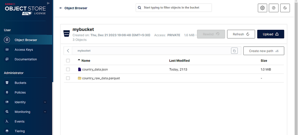Browsing contents of the bucket in MinIO (Image by author)

Here, you’ll find the earlier JSON file and the raw data in Parquet format.

Spark splits the Parquet data into multiple files in a folder, effectively chunking the data.

Now, let’s move on. We’ll transform the data as follows:

# Perform transformations to raw data
country_trnsfm_data = (
country_raw_data
.selectExpr(
"name.common as cntry_name",
"area as cntry_area",
"borders as border_cntry",
"capital as capital_cities",
"continents as cntry_continent",
"landlocked as is_landlocked",
"population",
"startOfWeek",
"timezones as nr_timezones",
"unMember as is_unmember"
)
.withColumn("cntry_area",F.when(F.col("cntry_area") < 0, None).otherwise(F.col("cntry_area")))
.withColumn("border_cntry",F.when(F.col("border_cntry").isNull(),F.array(F.lit("NA"))).otherwise(F.col("border_cntry")))
.withColumn("capital_cities",F.when(F.col("capital_cities").isNull(),F.array(F.lit("NA"))).otherwise(F.col("capital_cities")))
)

# Print schema of transformed data
country_trnsfm_data.printSchema()

Breaking down the code:

We select specific columns from the raw data for analysis. To access nested fields in this semi-structured data, we use the dot “.” operator.The cntry_area column is modified so that any negative value becomes NULL.For border_cntry and capital_cities, which are ArrayType, we replace NULL values with an array of NA.

After transformations, we’ll print the schema of the new dataframe.

root
|-- cntry_name: string (nullable = true)
|-- cntry_area: double (nullable = true)
|-- border_cntry: array (nullable = true)
| |-- element: string (containsNull = true)
|-- capital_cities: array (nullable = true)
| |-- element: string (containsNull = true)
|-- cntry_continent: array (nullable = true)
| |-- element: string (containsNull = true)
|-- is_landlocked: boolean (nullable = true)
|-- population: long (nullable = true)
|-- startOfWeek: string (nullable = true)
|-- nr_timezones: array (nullable = true)
| |-- element: string (containsNull = true)
|-- is_unmember: boolean (nullable = true)

Next, we’ll write the transformed data back as a new Parquet file.

# Write transformed data as PARQUET
country_trnsfm_data.write.mode("overwrite").format("parquet").save("s3a://mybucket/country_trnsfm_data.parquet")

Following that, we create an external Hive table over this Parquet file. Hive, a data warehouse software built on Hadoop, facilitates data querying and analysis. An external table means Hive only handles the metadata, with the actual data in an external location (our MinIO bucket).

# Create external hive table using PARQUET
spark.sql("""
CREATE EXTERNAL TABLE country_data (
cntry_name STRING,
cntry_area DOUBLE,
border_cntry ARRAY<STRING>,
capital_cities ARRAY<STRING>,
cntry_continent ARRAY<STRING>,
is_landlocked BOOLEAN,
population BIGINT,
startOfWeek STRING,
nr_timezones ARRAY<STRING>,
is_unmember BOOLEAN
)
STORED AS PARQUET
LOCATION 's3a://mybucket/country_trnsfm_data.parquet';
""").show()

Once our Hive table is ready, we can view its details with a specific command.

# Show table details
spark.sql("DESCRIBE EXTENDED default.country_data").show(100,truncate = False)

You’ll see the column names, data types, database name, location, table type, and more.

Now, let’s query the first five records from the table.

# Show first 5 records from the table
spark.sql("SELECT * FROM default.country_data LIMIT 5").show(truncate = False)

Next, we’ll read the table into a dataframe and create a temporary view on it. While it’s possible to query directly from the table, using temporary views on dataframes is common in Spark. Let’s explore that too.

# Create temporary view using dataframe
spark.table("default.country_data").createOrReplaceTempView("country_data_processed_view")

Fantastic. With this setup, we’re ready to start our analysis!

Analysing semi-structured data

Now comes the exciting part. Let’s dive into our data analysis by addressing some intriguing questions derived from our data. Here are the queries we aim to explore:

Which are the 10 largest countries in terms of area? (in sq. km.)Which country has the largest number of neighbouring countries?Which countries have the highest number of capital cities?How many countries lie on two or more continents?How many landlocked countries per continent?Which country has the highest number of time zones?How many countries are not UN members?

Knowing what we’re looking for, let’s start crafting some Spark SQL queries to uncover these insights. First, we’ll set up a utility function for displaying results in the notebook, saving us from repetitive coding.

# Function to show Spark SQL results
def show_results(sql_string):
return spark.sql(
sql_string
).show(truncate = False)

Let’s kick off with our initial query.

Q1. Which are the 10 largest countries in terms of area? (in sq. km.)

For this, we’ll arrange the data by the cntry_area column in descending order.

# 1. Which are the 10 largest countries in terms of area? (in sq. km.)
sql_string = """
SELECT cntry_name, cntry_area
FROM country_data_processed_view
ORDER BY cntry_area DESC
LIMIT 10
"""
show_results(sql_string)

+-------------+-----------+
|cntry_name |cntry_area |
+-------------+-----------+
|Russia |1.7098242E7|
|Antarctica |1.4E7 |
|Canada |9984670.0 |
|China |9706961.0 |
|United States|9372610.0 |
|Brazil |8515767.0 |
|Australia |7692024.0 |
|India |3287590.0 |
|Argentina |2780400.0 |
|Kazakhstan |2724900.0 |
+-------------+-----------+

We find that Russia has the largest area, followed by Antarctica. While there’s debate about Antarctica’s status as a country, it’s included in this dataset.

Q2. Which country has the largest number of neighbouring countries?

Next, we focus on the border_cntry column. It’s an array type listing the neighbouring countries’ codes for each country. By using the array_size function, we calculate the array lengths and order the data accordingly, excluding rows where border_cntry is NA.

# 2. Which country has the largest number of neighbouring countries?
sql_string = """
SELECT cntry_name, border_cntry, array_size(border_cntry) as ngbr_cntry_nr
FROM country_data_processed_view
WHERE NOT array_contains(border_cntry,'NA')
ORDER BY array_size(border_cntry) DESC
LIMIT 1
"""
show_results(sql_string)

+----------+--------------------------------------------------------------------------------+-------------+
|cntry_name|border_cntry |ngbr_cntry_nr|
+----------+--------------------------------------------------------------------------------+-------------+
|China |[AFG, BTN, MMR, HKG, IND, KAZ, NPL, PRK, KGZ, LAO, MAC, MNG, PAK, RUS, TJK, VNM]|16 |
+----------+--------------------------------------------------------------------------------+-------------+

This reveals China as the country with the most neighbours?—?a total of 16.

Q3. Which countries have the highest number of capital cities?

We’ll employ a similar method for the next question, applying array_size to the capital_cities column.

# 3. Which countries have the highest number of capital cities?
sql_string = """
SELECT cntry_name, capital_cities, array_size(capital_cities) as total_capital_cities
FROM country_data_processed_view
WHERE NOT array_contains(capital_cities,'NA')
ORDER BY array_size(capital_cities) DESC
LIMIT 2
"""
show_results(sql_string)

+------------+-----------------------------------+--------------------+
|cntry_name |capital_cities |total_capital_cities|
+------------+-----------------------------------+--------------------+
|South Africa|[Pretoria, Bloemfontein, Cape Town]|3 |
|Palestine |[Ramallah, Jerusalem] |2 |
+------------+-----------------------------------+--------------------+

The results highlight South Africa and Palestine as the only countries with multiple capital cities.

Q4. How many countries lie on two or more continents?

We’ll again use the array_size function, this time on the cntry_continent column.

# 4. How many countries lie on two or more continents?
sql_string = """
SELECT cntry_name, cntry_continent, array_size(cntry_continent) as total_continents
FROM country_data_processed_view
ORDER BY array_size(cntry_continent) DESC
LIMIT 3
"""
show_results(sql_string)

+----------+---------------+----------------+
|cntry_name|cntry_continent|total_continents|
+----------+---------------+----------------+
|Turkey |[Europe, Asia] |2 |
|Azerbaijan|[Europe, Asia] |2 |
|Russia |[Europe, Asia] |2 |
+----------+---------------+----------------+

It turns out Turkey, Azerbaijan, and Russia span two continents each?—?Europe and Asia.

Q5. How many landlocked countries per continent?

We’ll build a subquery with the country name, a boolean value indicating landlocked status, and an explode function for each cntry_continent array entry. Since a country may span multiple continents, we’ll aggregate by continent and sum the boolean values for landlocked countries.

# 5. How many landlocked countries per continent?
sql_string = """
SELECT continent, SUM(is_landlocked) as landlocked_nr
FROM (SELECT cntry_name, case when is_landlocked then 1 else 0 end as is_landlocked, explode(cntry_continent) as continent
FROM country_data_processed_view)
GROUP BY continent
ORDER BY SUM(is_landlocked) DESC
"""
show_results(sql_string)

+-------------+-------------+
|continent |landlocked_nr|
+-------------+-------------+
|Europe |16 |
|Africa |16 |
|Asia |12 |
|South America|2 |
|North America|0 |
|Antarctica |0 |
|Oceania |0 |
+-------------+-------------+

This indicates that Europe and Africa have the highest number of landlocked countries, considering a country may be counted more than once if it spans multiple continents.

Q6. Which country has the highest number of time zones?

Here, we use array_size on the nr_timezones column and sort the results in descending order.

# 6. Which country has the highest number of time zones?
sql_string = """
SELECT cntry_name, nr_timezones, array_size(nr_timezones) as total_timezones
FROM country_data_processed_view
ORDER BY array_size(nr_timezones) DESC
LIMIT 1
"""
show_results(sql_string)

+----------+----------------------------------------------------------------------------------------------------------------------------------------------------------+---------------+
|cntry_name|nr_timezones |total_timezones|
+----------+----------------------------------------------------------------------------------------------------------------------------------------------------------+---------------+
|France |[UTC-10:00, UTC-09:30, UTC-09:00, UTC-08:00, UTC-04:00, UTC-03:00, UTC+01:00, UTC+02:00, UTC+03:00, UTC+04:00, UTC+05:00, UTC+10:00, UTC+11:00, UTC+12:00]|14 |
+----------+----------------------------------------------------------------------------------------------------------------------------------------------------------+---------------+

Interestingly, France tops the list, likely due to its territories beyond mainland France.

Q7. How many countries are not UN members?

Here, we count the number of countries where is_unmember is False.

# 7. How many countries are not UN members?
sql_string = """
SELECT COUNT(*) AS count
FROM country_data_processed_view
WHERE NOT is_unmember
"""
show_results(sql_string)

+-----+
|count|
+-----+
|57 |
+-----+

According to the dataset, 57 countries are not UN members, a figure that includes independent territories and regions classified as countries. You can find the complete notebook here.

That wraps up our analysis! But before concluding, let’s discuss how to properly clean up our resources.

Cleanup of resources

After finishing, don’t forget to save your notebook. Then, it’s time to stop the Docker containers. In the Docker Desktop app, just click the stop button.

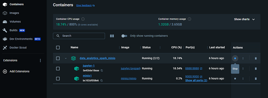Stopping all the containers at once (Image by author)

This action will halt both containers simultaneously. Alternatively, you can stop each container one by one. You can choose to either retain these containers or delete them.

Be aware, deleting the JupyterLab container means losing your notebook, as a new JupyterLab instance starts from scratch. However, your MinIO data will stay intact, as it’s stored on your host machine, not in the container’s memory.

If you choose to remove the containers, you might also want to delete the Docker images for JupyterLab and MinIO, especially if you’re tight on storage. You can do this in the “Images” section of the Docker Desktop app.

Conclusion

In this story, we explored a straightforward yet captivating data analytics case. We began by configuring our environment using Docker Compose. Next, we fetched data from an API, mimicking a real-world scenario. We then saved this data in a bucket similar to Amazon S3, in JSON format. Using PySpark, we enhanced this data and stored it persistently in Parquet format. We also learned how to create an external Hive table on top of this data. Finally, we used this table for our analysis, which involved working with complex data types like arrays.

I sincerely hope this guide was beneficial for you. Should you have any questions, please don’t hesitate to drop them in the comments below.

References

GitHub repository: https://github.com/sarthak-sarbahi/data-analytics-minio-spark/tree/mainDocker Compose: https://docs.docker.com/compose/MinIO: https://min.io/docs/minio/linux/index.htmlPySpark: https://spark.apache.org/docs/latest/api/python/index.html

---

Seamless Data Analytics Workflow: From Dockerized JupyterLab and MinIO to Insights with Spark SQL was originally published in Towards Data Science on Medium, where people are continuing the conversation by highlighting and responding to this story.

---

View Entire Post